The Quest
Since mid-August my home/office floor has been vibrating. Like a refrigerator/air conditioner compressor that rumbles 24/7. It’s insidious - can’t sleep, can’t focus on work, sometimes it makes me sea sick. Stayed in a hotel for a week just to regain my sanity.
There was a lot of work in this old building the past 4 months. I’ve talked to the builders and building management, but that led to no solutions. The surrounding neighbors turned off their power at the breaker to help isolate it, but it doesn’t seem to be coming from them or I’m so used to it I can’t tell when it stops.
If only for my own sanity I’ve been trying to measure the vibration and maybe find out where it is most intense.
- I tried an accelerometer but cheap XYZ accelerometers aren’t sensitive enough to capture it clearly.
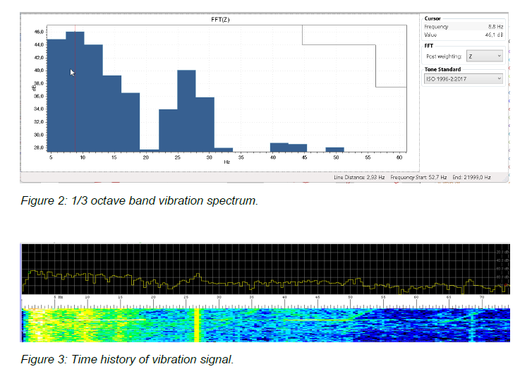
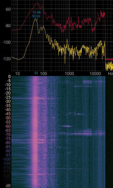
- I tried several audio spectrograms, but it’s a vibration not a noise. I think I see resonate frequencies produced by the vibration, compared to say the quiet room of the library, but I’m not certain. The 47kHz line seems to be coming from the phone itself, its always present even outdoors on a quiet night.
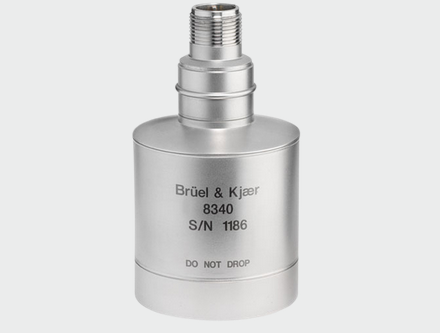
Seismic accelerometer
This led me to the world of high-powered microscope installation, industrial vibration analysis and amateur seismology. The two options seem to be:
- A seismic accelerometer used in building construction to spot dangerous vibrations before they cause severe damage.
- A geophone, an analog sensor that can measure earthquakes thousands of miles away and traffic passing on the road outside.
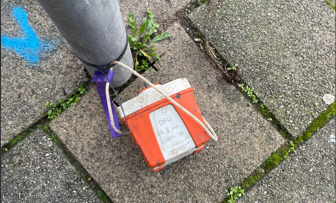
The Geophone
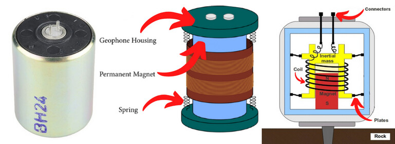
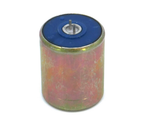
Geophone
Seismic accelerometers are very expensive, so let’s look at geophones. Geophones are magnets inside a metal coil that produce a voltage when the magnet shakes.
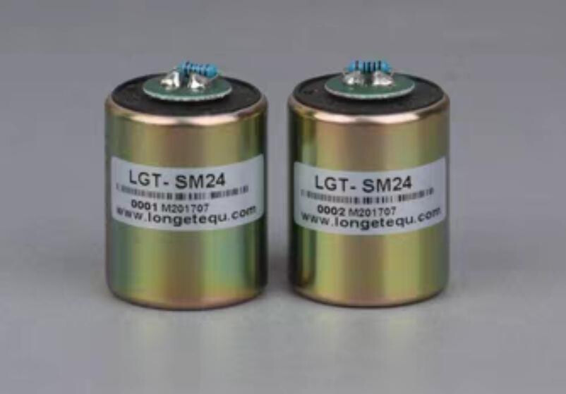
This is the SM-24, which seems to be similar in specs to the geophone SparkFun sold at one point for $69 (vs $10 on Taobao…).
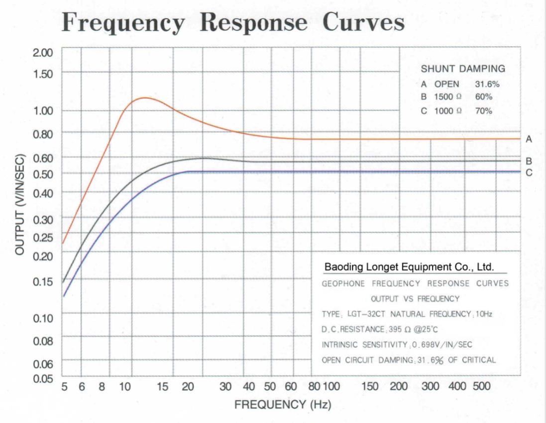
Parameter Seismic Geophones:
| Parameter | LGT-SM24 | LGT-SM24/H |
|---|---|---|
| Natural frequency (Hz) | 10±2.5% | 10±2.5% |
| Open circuit damping | 0.25±2.5% | 0.271±2.5% |
| Closed circuit damping | 0.6±5% (1339R) 0.6±2.5% |
0.6±2.5% |
| Open circuit sensitivity (V/cm/s) | 0.686±5% (1000R) 0.288±2.5% |
0.288±2.5% |
| Closed circuit sensitivity (V/cm/s) | 0.225±5% (1339R) 0.209±5% (1000R) |
0.227±2.5% |
| Open circuit resistance (Ω) | 375±2.5% | 375±2.5% |
| Closed circuit resistance (Ω) | 293 or 273 | 296±2.5% |
| Distortion | ≤0.1% | ≤0.1% |
| Transverse natural frequency (Hz) | ≥250 | ≥250 |
| Overall mass (g) | 11 | 11.3 |
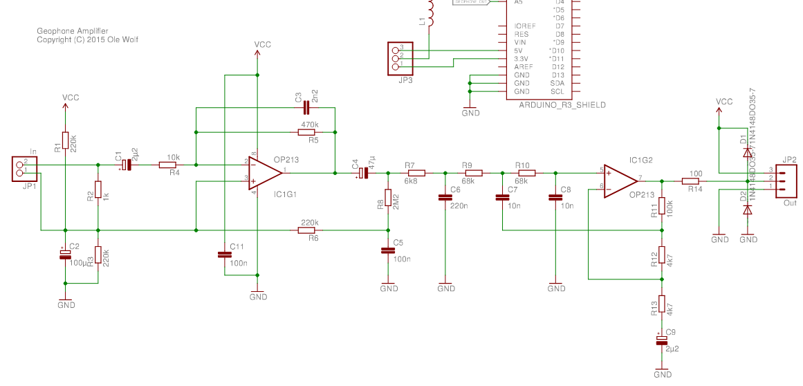
The Amplification
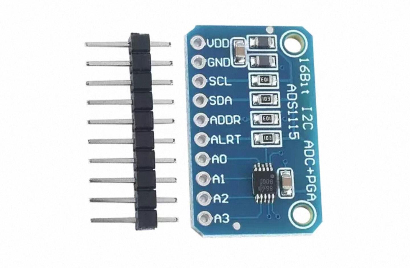
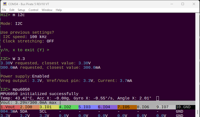
Geophones make a tiny voltage when measuring something like an earthquake 2000km away. Amateur seismology devices use an op-amp to amplify the voltage, and tend to use high resolution ADCs (24bits+). However the gain doesn’t seem to be that significant, this example only uses a ADS1115 16bit I2C ADC with programmable 1-16x gain, and that seems sufficient. In comparison, the current measurement on the Bus Pirate uses a gain of 32+.
For something like foot step detection (or a vibrating floor) amplification may not be needed. We’ll experiment to find out ![]() I picked up:
I picked up:
- ADS1115 programmable gain ADC
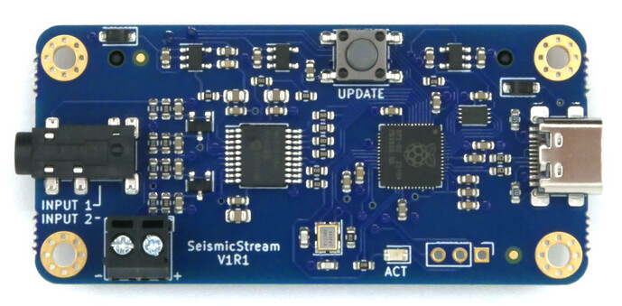
- Seismic Stream which evidently has a pretty good filter and uses the RP2040.
The Analysis
Most amateur seismograph applications are happy with a simple voltage/time graph. I actually need to identify the dominant frequency. Analysis has been a sticking point on this misery mystery tour - until yesterday.
Vibration research has several good resources about vibration measurement. This post on fast Fourier transform vs Power Spectral Density was the clue I needed to move forward.
Enter endaq which has an open source Python library for vibration analysis. The library is kind of outdated:
- Must use Python 3.11 so it works with numpy<2.0
- Must use numpy < 2.0
- Must use plotly>=5.15.0
- Comment out #endaq.plot.utilities.set_theme(‘endaq’)
The code for the tutorial is in some kind of Google virtual dev environment, which doesn’t work because the default packages are all too new. I’ve copy and pasted the code snippets below:
endaq Python examples
import endaq
#numpy<2.0" "plotly>=5.15.0
import plotly.express as px
import plotly.graph_objects as go
import numpy as np
import pandas as pd
import scipy
import os
#endaq.plot.utilities.set_theme('endaq')
# Create plots directory if it doesn't exist
os.makedirs('plots', exist_ok=True)
def save_plot(fig, name):
fig.write_html('plots/'+name+'.html', include_plotlyjs='cdn')
fig.write_image('plots/'+name+'.png')
fig.write_image('plots/'+name+'.svg')
"""Generate Sample Data"""
# Get a Random Signal with Frequency Content Between 10 and 50 Hz
noise = endaq.calc.filters.band_limited_noise(min_freq=10, max_freq=50, duration=10, sample_rate=250, norm='rms')
# Add a Column with a Simple Sine Wave
noise['30 & 80.25 Hz Sine Wave'] = np.sin(noise.index * 2 * np.pi * 30) + np.sin(noise.index * 2 * np.pi * 80.25)
# Add a Column with Both
noise['Sine on Random'] = noise['30 & 80.25 Hz Sine Wave'] + noise['Noise from 10 to 50 Hz']
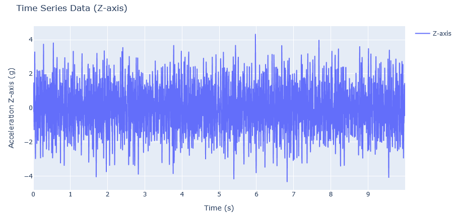
"""Plot Time Series"""
fig = px.line(noise).update_layout(yaxis_title_text='Acceleration (g)', legend_title_text='')
save_plot(fig, '1_noise_time_series')
fig.show()
"""Calculate PSD with Function"""
psd = endaq.calc.psd.welch(noise, bin_width=1)
psd
"""Plot PSD"""
fig = px.line(psd).update_layout(
yaxis_title_text='Acceleration (g^2/Hz)',
xaxis_title_text='Frequency (Hz)',
legend_title_text='')
save_plot(fig, '2_noise_psd')
fig.show()
"""Various durations and bin widths"""
psd = pd.DataFrame()
for t in [1, 1.1, 2, 8, 9, 10]:
psd_t = endaq.calc.psd.welch(noise[:t], bin_width=0.5).reset_index().melt(id_vars='frequency (Hz)')
psd_t.columns = ['Frequency (Hz)', 'variable', 'value']
psd_t['Time'] = '0 to ' + str(t)
psd_t['Bin Width'] = '0.5 Hz'
psd_t2 = endaq.calc.psd.welch(noise[:t], bin_width=1).reset_index().melt(id_vars='frequency (Hz)')
psd_t2.columns = ['Frequency (Hz)', 'variable', 'value']
psd_t2['Time'] = '0 to ' + str(t)
psd_t2['Bin Width'] = '1 Hz'
psd_t3 = endaq.calc.psd.welch(noise[:t], bin_width=2).reset_index().melt(id_vars='frequency (Hz)')
psd_t3.columns = ['Frequency (Hz)', 'variable', 'value']
psd_t3['Time'] = '0 to ' + str(t)
psd_t3['Bin Width'] = '2 Hz'
psd = pd.concat([psd, psd_t, psd_t2, psd_t3])
fig = px.line(
psd,
x='Frequency (Hz)',
y='value',
facet_col='variable',
facet_col_spacing=0.03,
facet_row='Bin Width',
color='Time'
)
fig.for_each_annotation(lambda a: a.update(text=a.text.split("=")[-1]))
fig.update_yaxes(showticklabels=True, matches='y', title_text='')
for i in range(0,3):
fig.update_yaxes(showticklabels=True, matches=f'y{i+1}', col=i+1)
fig.update_layout(title_text='PSD of Varying Lengths (Amplitude^2/Hz vs Frequency)')
save_plot(fig, '3_noise_psd_length_bin')
fig.show()
"""Demonstrate time segments"""
segments = pd.DataFrame()
for s in np.arange(19)/2:
df = noise[['Noise from 10 to 50 Hz']][s:s+1]
window = scipy.signal.windows.hann(len(df))
df = df.mul(window, axis="rows")
df['Center Time'] = s + 0.5
segments = pd.concat([segments, df.reset_index()])
fig = px.line(
segments,
x='Time (s)',
y='Noise from 10 to 50 Hz',
color='Center Time'
).update_layout(title_text='Overlapping Segments with Hanning Window Applied')
save_plot(fig, '4_windows')
fig.show()
"""Compute FFTs for Each Segment"""
ffts = pd.DataFrame()
for t in segments['Center Time'].unique():
df = segments[segments['Center Time'] == t][['Time (s)', 'Noise from 10 to 50 Hz']].set_index('Time (s)')
df.columns = [t]
fft = endaq.calc.fft.rfft(df.iloc[1:]).reset_index().melt(id_vars='frequency (Hz)')
ffts = pd.concat([ffts, fft])
ffts['var'] = 'var'
ffts.variable = ffts.variable.astype(float)
waterfall = endaq.plot.spectrum_over_time(
ffts, plot_type='Waterfall',
var_column='var', time_column='variable')
save_plot(waterfall, '5_waterfall')
waterfall.show()
"""Square, Normalize, and Convert to PSD Units"""
ffts['frequency (Hz)'] = np.round(ffts['frequency (Hz)'],1)
spec = ffts.pivot_table(index='frequency (Hz)',columns='variable',values='value')
psd = spec ** 2 # square
psd = psd / psd.index[1] # divide by bin width
psd = psd * 1.333 # deal with scaling due to windowing
from plotly import colors
color_sequence = colors.sample_colorscale(
[[0.0, '#6914F0'],
[0.2, '#3764FF'],
[0.4, '#2DB473'],
[0.6, '#FAC85F'],
[0.8, '#EE7F27'],
[1.0, '#D72D2D']], len(psd.columns))
fig = px.line(
psd,
color_discrete_sequence=color_sequence
).update_layout(yaxis_title_text='Amplitude ** 2 / Hz', xaxis_title_text='Frequency (Hz)', legend_title_text='')
fig.add_trace(go.Scattergl(
x=psd.index,
y=psd.mean(axis=1).to_numpy(),
name='Average of All Segments',
mode='lines',
line_width=10,
line_color='gray'
))
save_plot(fig, '6_psd_segments')
fig.show()
"""Using Spectrogram Function"""
spectrogram = endaq.calc.psd.rolling_psd(noise, bin_width=1, num_slices=20, add_resultant=False)
spectrogram
fig = px.line(
spec,
color_discrete_sequence=color_sequence
).update_layout(yaxis_title_text='Amplitude ** 2 / Hz', xaxis_title_text='Frequency (Hz)', legend_title_text='')
fig.add_trace(go.Scattergl(
x=spec.index,
y=spec.mean(axis=1).to_numpy(),
name='Average of All Segments',
mode='lines',
line_width=10,
line_color='gray'
))
save_plot(fig, '7_psd_segments_from_spectrogram')
fig.show()
animation = endaq.plot.spectrum_over_time(spectrogram, plot_type='Animation')
save_plot(fig, '8_animation')
animation.show()
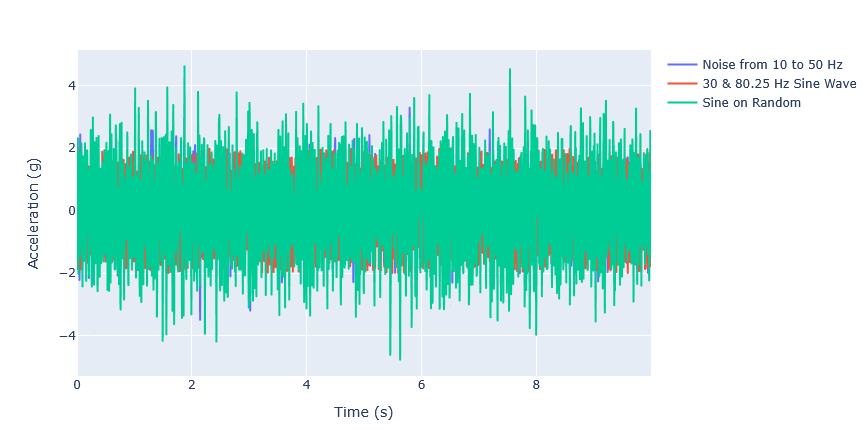
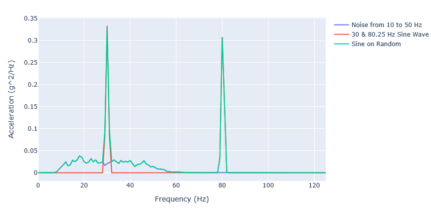
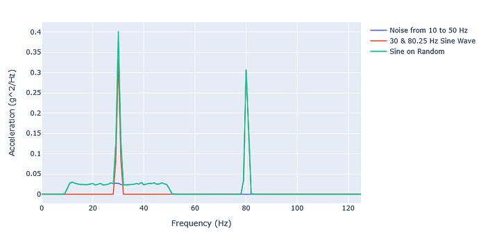
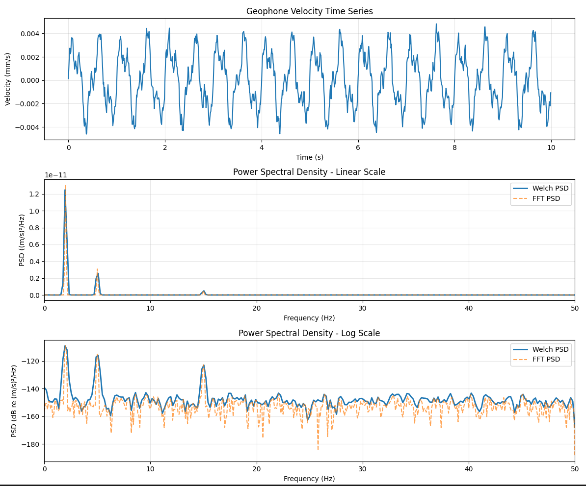
The example creates this signal with lots of noise and no obvious major frequency component.
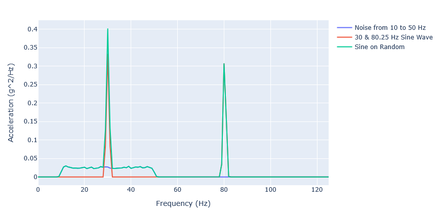
Through PSD analysis the major frequency components are obvious. That’s some good analysis!
The Goals
- Simply visualize/confirm that there is a vibration here that isn’t present in surrounding buildings. Have some actual data so I’m more than a mad man ranting about the walls closing in on me.
- Hopefully get some idea of the frequency and strength, which might lead to finding the cause.
- Maybe locate where it is strongest, the direction it’s coming from
- Do another round of turning off power around the building, but this time with actual data to see if the vibration stops
- If confirmed, and I can’t spur any action, I found a consultancy which will use a calibrated geophone and provide a “legally valid” report. There are regulations covering occupational vibration limits, and I’m pretty sure residential as well, so I could use that as a basis to request further action. More research needed here, hopefully we can
DUIDIY (ED: too funny, leaving it in) our way out of this mystery.
Thank you for attending my TED talk.